Environment Information Detection

David Zikel

Problem and motivation

Detection of ambient weather and climate conditions from a single image is useful in automatically categorizing images, such as on image uploading sites like Flickr. Many of these attributes can be detected through new techniques or novel applications of existing ones. This project, using various analysis methods including retinex single-image lighting approximation, automatically categorizes images based on several ambient attributes: fog, time of day, and approximate temperature.

Edge detection:

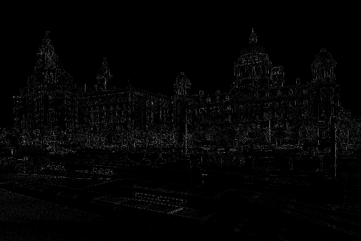The amount of fog in an image can be estimated by measuring the intensity of edges in the image. In an image with no fog, the edges should be strong, and, conversely, in an image with prevalent fog, the edges should be weak. To measure the strength of an image’s edges, a modified version of a standard edge detection algorithm can be used.

For this project, an image’s edges are first detected (as a binary output, EDGE or NOT EDGE, per pixel) using the Canny edge detection algorithm. For each edge pixel detected by the Canny algorithm, the program analyzes a small (21x21) neighborhood of that edge to find the edge point in that region furthest from the original pixel. It is assumed, and this assumption has proven accurate in all analyzed images of actual scenes, that the line from the initial pixel to the found pixel is tangent to the line formed by all edge pixels.

Given this tangent line, color values are taken from two locations in the (original, color) image, both offset from the initial edge pixel in a direction perpendicular to the found tangent. This, in effect, finds the color of the image on each side of the edge being analyzed. The distance between these colors is computed (treating colors as coordinates in RGB-space), and the intensity of the edge pixel is returned as this distance.

For measuring fog, it suffices to take the average edge intensity among all pixels detected by the Canny algorithm as edges. If this average intensity is above a certain threshold, it can be assumed that there is no major fog - conversely, if the intensity is below this threshold, fog is noticeable in the image. Using this modified Canny algorithm, images had significant fog if and only if their average measured edge intensity was less than 0.2.

Skyline detection:

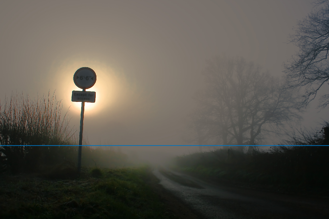For determining the color balance of parts of an image, it is beneficial to find the location of the skyline or horizon line - the vertical position in the image marking the divide between the sky (or a very far-off part of the scene) and the objects being photographed. If the camera is aligned horizontally, this skyline will always be a horizontal line across the image. This means that, for the purposes of computation, only a y-coordinate must be found.

The ‘skyline’ is modeled as the point along the image (vertically) such that the image is closest in the \(L^2\) norm to a step function on the y coordinate with its step located along the skyline. Equivalently, modeling the image as a function \(f : [0,1] \times [0,1] \rightarrow [0,1]\), the skyline position is the value \(\hat{y}\) such that the minimum value of

\[\int_{0}^{1} \int_{0}^{1} (f(x,y) - \mu(y))^2\,dx\,dy\]

across all functions

\[\mu(y) = \cases{\mu_u \quad y < \hat{y} \\ \mu_d \quad y \geq \hat{y}}\]

is the minimum across all step functions \(\mu\). (For images with multiple color channels, the squared errors for each channel are summed to find the final result.)

It is clear that the values of \(\mu_u\) and \(\mu_d\) minimizing this integral for a given \(\hat{y}\) are simply the average values of the image function \(f\) across \(y \in [0,\hat{y}]\) and \(y \in (\hat{y},1]\) respectively. Using these values for the outputs of \(\mu\), \(\hat{y}\) can be found to pixel precision by testing every value of \(y\) corresponding to a pixel location. The computation of one such sum of squared errors per column can be done almost instantaneously, even for large images, by precomputing the sum and sum-of-squares of each row (allowing for immediate computation of these sums for the upper and lower portions of the image), treating the squared-error calculation as the computation of a variance, and observing that \(\sigma^2 = \langle (X - \langle X \rangle)^2 \rangle = \langle X^2 \rangle - {\langle X \rangle}^2\).

Lighting data

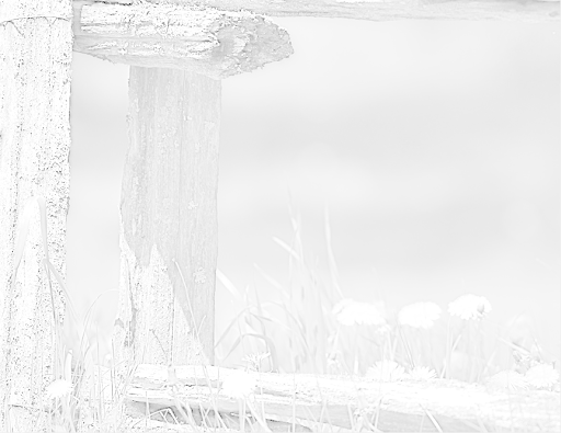
To estimate lighting, the program uses retinex-based approximations to the lighting image. The main source of the algorithm is the first paper cited, “A Variational Framework for Retinex” (https://www.cs.technion.ac.il/~ron/PAPERS/retinex_ijcv2003.pdf). The algorithm implemented is based on the assumption, accurate outside of scenes with highly reflective surfaces, that every object in the scene has a visible brightness proportional to the product of a global lighting value and a local reflectance value (the latter less than 1).

Algorithm principles

Lighting approximation algorithms attempt to extract two images from one input image. These images are a lighting image, which contains the ambient light information for a scene, and an albedo image, which contains the innate reflectance information for all objects in that scene. These output images are directly and algorithm-independently linked to the input image in two ways: the first is that the lighting image is always as bright as or brighter than the input image, and the second is that the per-pixel product of the lighting and albedo images is equal to the input image.

The most prominent attribute of real lighting data, and the attribute lighting extraction algorithms most heavily rely on, is the smoothness of the lighting intensity across space. Two other properties of the lighting data are used to fine-tune the initial lighting estimate, using penalty parameters which are provided as input to the algorithm. The first property is that the lighting image should relatively closely resemble the input image, and the second property is that the albedo image (input divided by lighting) should, like the lighting image, be spatially smooth. A penalty formula is created based on these three attributes, and its solution is found using gradient descent.

Algorithm details

All computations in the retinex algorithm are done on the logarithm of the input image, and the output is the logarithm of the lighting image, for two reasons. The first is mathematical convenience - rather than requiring divisions for each pixel to compute the albedo image for the third penalty term, the algorithm will only use subtractions. The second reason is that a logarithmic scale more closely approximates the way humans consider lighting. For instance, the most common means of brightening an image, gamma correction, raises the intensity value for each pixel to a fixed exponent rather than using additive or multiplicative scaling.

Denoting the (logarithm of the) original image by \(S\) and the (logarithm of the) current lighting image by \(L\), three penalty terms are computed, corresponding to the three criteria on \(L\) specified above:

\(\|\nabla L\|^2\) for smoothness,

\(\alpha (L-S)^2\) for proximity, and

\(\beta \|\nabla (L-S)\|^2\) for albedo smoothness.

The total penalty integral over image space \(I\), then, is \(\int \int_{I} (\|\nabla L\|^2 + \alpha (L-S)^2 + \beta \|\nabla (L-S)\|^2) \,dx \,dy\). If is is assumed that \(\nabla S = \nabla L = 0\) on the boundary of \(I\), this integral simplifies to \(\int \int_{I} (-L \Delta L + \alpha (L-S)^2 - \beta (L-S) \Delta (L-S)) \,dx \,dy\), where \(\Delta\) is the Laplacian operator \(\nabla \cdot \nabla\).

For performance, the initial steps of the algorithm are run on smaller copies of the original image. Each copy is made from the copy of the next largest size by taking weighted averages of points at certain coordinates, approximating Gaussian weights as these averages are iterated. In the algorithm as implemented, 40 percent of gradient descent iterations are run on an image 1/64 the size of the original input (1/8 scale along both axes), 30 percent on an image 1/16 the size, 20 percent on an image 1/4 the size, and only 10% of iterations on the original input. As, due to the smoothness requirement, the most important attributes of the lighting image are its large-scale properties, this process greatly speeds up convergence.

Gradient descent

The penalty function is treated as a function from the space of one-color images to the real numbers. Its gradient can easily be computed as \(G = 2(-\Delta L + \alpha (L - S) - \beta \Delta (L - S))\). The gradient is the direction of steepest ascent for any multivariate function, so the negative of the gradient is the direction of steepest descent. As such, the algorithm replaces \(L\) with \(L - \mu G\) for some scaling factor \(\mu\).

To find an optimal value for \(\mu\), several simplifications can be made: the best value for \(\mu\) minimizes the penalty function on the line in the direction of \(G\), which makes the derivative along this line equal to 0, so Newton’s method can be used to find an approximate zero for this derivative. The derivative along this line at \(L\) is simply \(G \cdot G\), and the second derivative can be computed as \(\alpha G \cdot G - (1 + \beta) G \cdot \Delta G\), where the \(\Delta\) operation is taken along the two image coordinates and not the many ‘coordinates’ in the space of images.

The estimated step \(\mu\), then, is calculated as \(\frac{G \cdot G}{\alpha G \cdot G - (1 + \beta) G \cdot \Delta G}\). The image \(L\), likewise, is updated to equal \(L - \mu G\). The final step per iteration is to project \(L\) onto the space of valid lighting approximations by, for every pixel of \(L\), setting its brightness to the larger of its current brightness and the brightness of the corresponding point in \(S\).

Data aggregation

The data returned consists of four fields:

• fog, a numeric value measuring the approximate amount of fog in the scene,
• fog_str, a string categorizing this level of fog,
• time, a numeric value measuring brightness as it corresponds to the time of day,
• time_str, categorizing time,
• warmth, a numeric value measuring the approximate temperature of the image (specifically, its color balance), and
• warmth_str, categorizing warmth.

fog is computed simply, as discussed in the section on edge detection - its value is one minus the average edge intensity. fog_str indicates fog if this value exceeds 0.8, and high fog if it exceeds 0.9. time is the average intensity of the color red below the estimated horizon line, and time_str categorizes this as night for values less than 0.2, day for values at least 0.5, and as midday or artificially brightly lit for values between 0.2 and 0.5. warmth - a measurement intrinsically less accurate than the others, as temperature does not leave major visible traces on images and can be further confounded by effects such as windchill - measures the warmth of the image’s color scheme and contains the difference between the average lighting red and blue intensities below the horizon line, with warmth_str categorizing this as warm if the value is positive and as cool otherwise.

Much of the raw data used in these computations - the edge intensity image, the horizon line location, and the retinex lighting images - is also immediately understandable to an end user. As such, these images (6 in all - edge intensity, horizon location, lighting for average colors, and lighting for each color channel) can be displayed directly to the user during the computation process. They can be useful for more subjective interpretations of an image’s lighting, or by niche users for estimating (by eye) specific attributes of the lighting or edge intensity which do not relate to climate for the purpose of categorization.

Citations

“A Variational Framework for Retinex”, Kimmel, Elad, Shaked, Keshet, and Sobel, 2003. https://www.cs.technion.ac.il/~ron/PAPERS/retinex_ijcv2003.pdf (primary source of algorithm implemented)

“Computational Color Science”, chapter 3, Provenzi, 2017. https://onlinelibrary-wiley-com.ezproxy.library.wisc.edu/doi/pdfdirect/10.1002/9781119407416

“STAR: A Structure and Texture Aware Retinex Model”, Xu, Hou, Ren, Liu, Zhu, Yu, Wang, and Shao, 2020. https://arxiv.org/pdf/1906.06690.pdf

Class submissions

Proposal: Link

Midterm report: Link

Presentation: Link